Efficient pretraining with token superposition

TL;DR. A 2–3× wall-clock speedup on LLM pretraining at matched FLOPs, without changing the final model architecture, optimizer, tokenizer, or training data. During the first 20–40% of training, the model reads and predicts bags of $s$ contiguous tokens — averaging their embeddings on the input side, predicting the next bag with a modified cross-entropy on the output side. For the remainder of the run, it trains normally on next-token prediction. The inference-time model is identical to one produced by conventional pretraining. Validated at 270M, 600M, and 3B dense, and at 10B-A1B MoE.

We introduce Token Superposition Training (TST), a modification to the standard LLM pretraining loop that produces substantial wall-clock speedups at fixed compute, without requiring any change to the model architecture, the optimizer, the parallelism strategy, the tokenizer, or the training data. On a 10B-A1B mixture-of-experts model trained to 2T tokens, TST reaches a lower final training loss than a matched-FLOPs baseline in roughly 40% of the wall-clock, and beats that baseline on HellaSwag, ARC-Easy, ARC-Challenge, and MMLU. The method consists of two phases: an initial superposition phase in which the model processes and predicts contiguous bags of tokens rather than individual tokens, and a recovery phase in which it returns to ordinary next-token training for the remainder of the run. The resulting model, at inference time, is identical in every respect to a model produced by conventional pretraining. Only the training loop changes.

The idea is motivated by a pair of observations about where pretraining efficiency comes from in the first place. It has been understood for some time that the performance advantage of subword tokenization over byte-level modeling is not, as sometimes claimed, primarily a matter of learned semantic structure. Work by Gigant et al. and concurrent studies on subword-to-byte distillation (Minixhofer et al.) and proxy compression (Zheng et al.) suggest that a large fraction of the BPE advantage at isoFLOPs comes simply from the fact that subword sequences are shorter, and the model therefore sees more natural-language content per unit of compute. If that is the case, then pretraining efficiency is at least partly a throughput problem, and one can ask whether the throughput lever can be pulled independently of the tokenizer.

The second observation concerns the relationship between training-time and inference-time efficiency. Recent work on chain-of-thought reasoning, ParScale, looped language models, and speculative decoding has shown that the two can be scaled separately: it is possible to spend more compute at inference than at training, and to improve downstream task performance by doing so. The same decoupling has received less attention in the other direction. Most efforts to improve pretraining efficiency, whether through sparse attention, mixture-of-experts, or alternative tokenizations, simultaneously change the trained artifact. This coupling makes comparisons difficult, introduces confounds between training-time and inference-time gains, and in some cases cancels the training savings against a slower or less capable inference model. We therefore adopt a stricter criterion: any method we are willing to call a pretraining efficiency improvement must leave the inference-time architecture untouched.

The question that follows is whether a training-time-only intervention can substantially increase token throughput at isoFLOPs while preserving the final model. This paper argues that it can, and that a surprisingly simple one works.

The method

The method is basically just a reshape, a mean, and a summed cross-entropy.

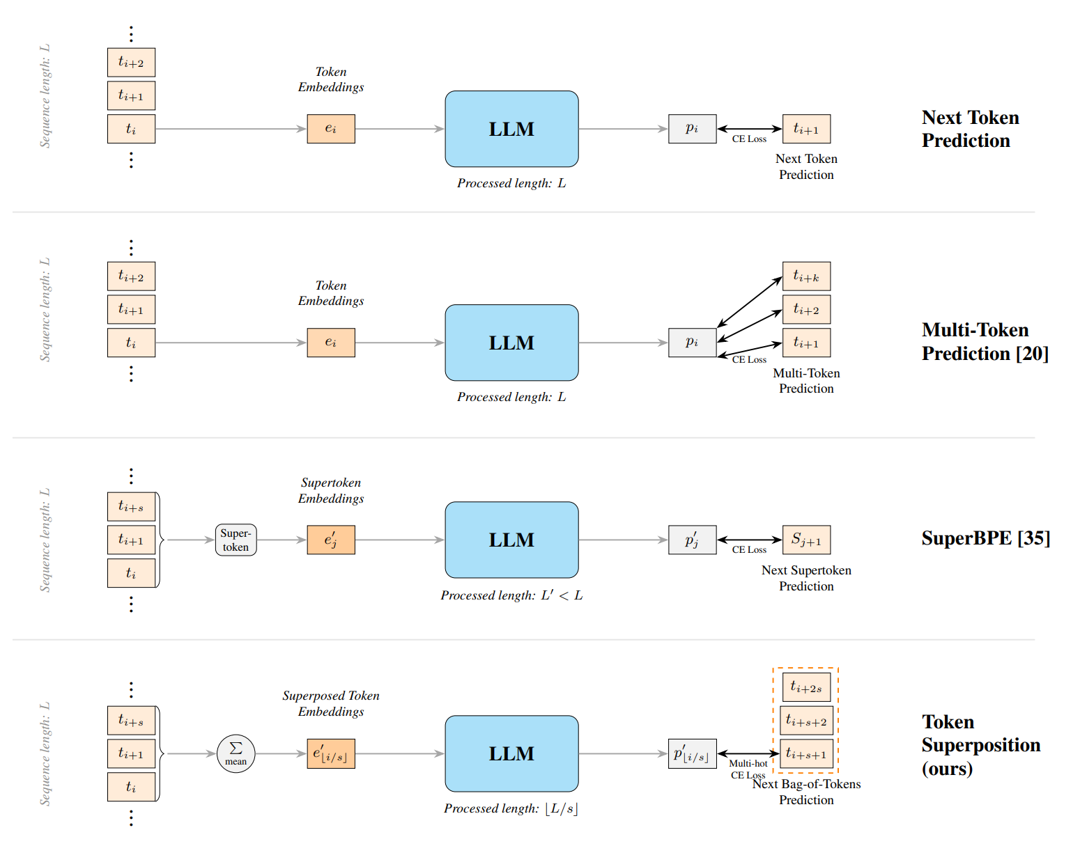
The two modifications TST introduces to standard causal language modeling are as follows. During the superposition phase, we segment the input sequence of length $L = l \cdot s$ into $l$ non-overlapping bags of $s$ contiguous tokens, and replace each bag in the embedding layer with the mean of the $s$ token embeddings:

$$ e'_{\lfloor i/s \rfloor} \;=\; \frac{1}{s} \sum_{k=0}^{s-1} e_{\lfloor i/s \rfloor \cdot s + k} $$

The transformer then processes a sequence of length $l$, while the underlying text corresponds to $L$ tokens. In PyTorch the input-side change is a reshape:

if superposition_bag_size > 1:
    bs, seq = inputs.shape
    # (bs, seq) -> (bs, seq // s, s)
    inputs = inputs.reshape(bs, seq // superposition_bag_size, superposition_bag_size)

followed by a mean over the new trailing axis in the embedding lookup. Nothing else in the forward pass changes. Because each latent position corresponds to $s$ source tokens, the model processes $s$ times as much text per unit of work as it would under standard training.

At each latent position $k$, the target is the next bag of tokens, and the loss is a mean cross-entropy over the $s$ targets:

$$ \mathcal{L}_{\text{MCE}}(\mathbf{z}, \mathbf{y}) \;=\; \frac{1}{s}\sum_{y \in \mathbf{y}} \mathcal{L}_{\text{CE}}(\mathbf{z}, y) $$

This can be derived from a multi-hot cross-entropy where each valid target token receives probability mass $1/s$; the equivalence is worked out in detail in Appendix B of the paper. The important consequence is that the MCE loss reduces to a sum of ordinary CE terms, which means an implementation can reuse the fused cross-entropy kernel already present in any major pretraining library. There is no new kernel to write, no auxiliary head to add, no change to the output projection.

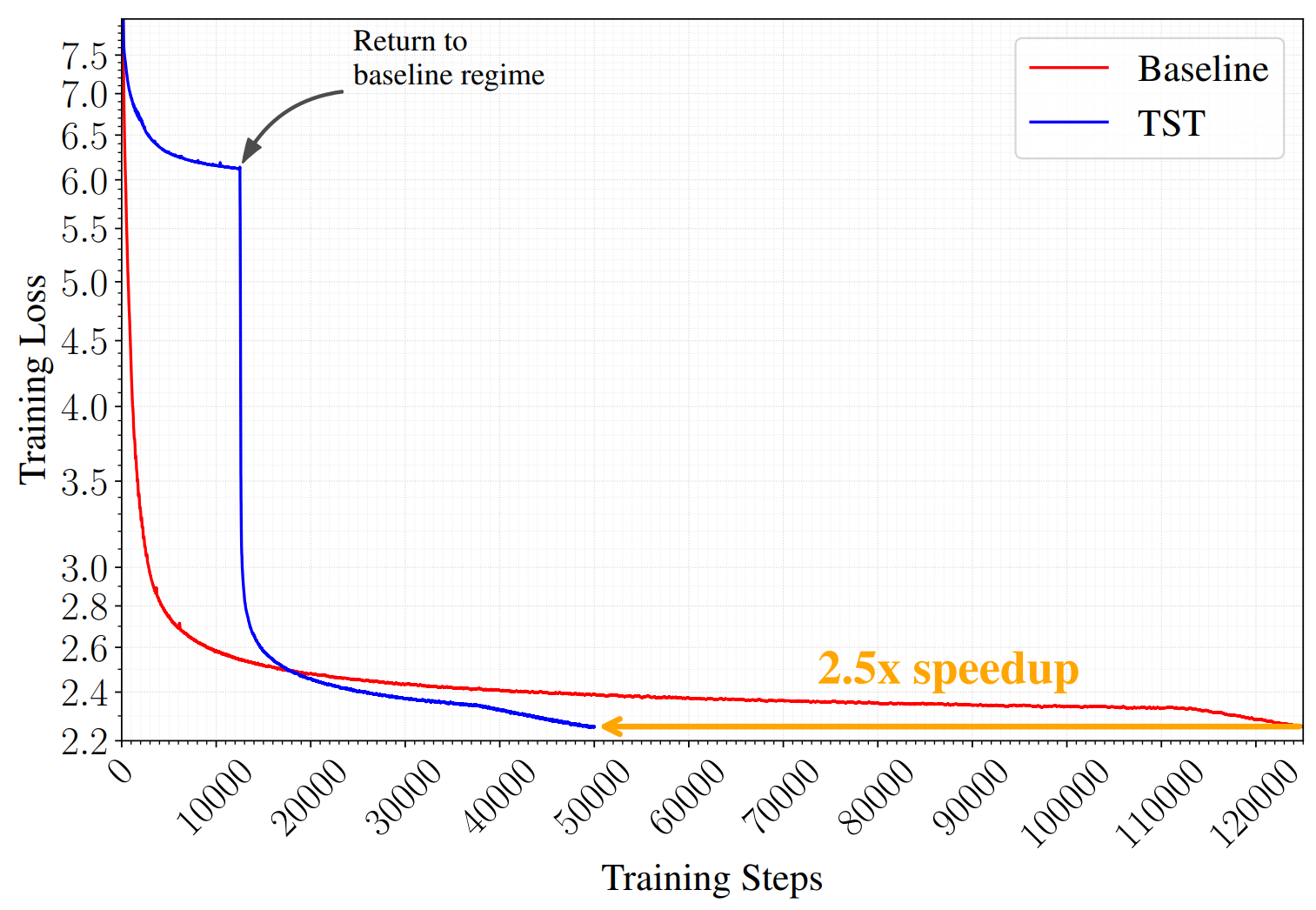
The objective is semi-autoregressive. The model still reads left to right across latent positions, but within each bag the ordering of the $s$ tokens is discarded, and sampling at inference produces mixed distributions over $s$ future positions that read as noise. A model trained only under this objective is not a usable next-token model. To recover one, we train under the superposition objective for a fraction $r$ of the total steps and then resume from the checkpoint under the standard next-token loss for the remaining $1 - r$. The loss curve shows a spike at the transition, typically between 1 and 2 nats, which resolves within a few thousand steps; the recovered model then crosses below the baseline and remains there for the rest of the run.

Two hyperparameters control the method: the bag size $s$ and the step ratio $r$. We will return to their sensitivity in the experimental section, but the short version is that any $r$ in $[0.2, 0.4]$ is close to optimal at the scales we studied, and $s$ has a flat-bottomed optimum whose location drifts upward with model size.

Experiments

Matched loss at roughly half the wall-clock on the 3B and 10B runs, consistent across four model scales. The optimal bag size grows with model size.

We train at four scales: 270M and 600M dense (both modified SmolLM2 shapes with untied embeddings and the Llama3-8B tokenizer), 3B dense (SmolLM3 shape), and a 10B-A1B mixture-of-experts in the Qwen3 family. Data is DCLM for the small runs and a 50/50 DCLM / FineWeb-Edu mix for the MoE. All models use AdamW with the Warmup-Stable-Decay schedule; learning rates are swept at 270M and 600M and taken from the respective family's recommendation at 3B and 10B. Training is done in TorchTitan under FSDP on up to 64 B200 GPUs. The full configuration table is in Appendix A of the paper.

A TST run admits three natural comparisons against its baseline, shown in Figure 3. At matched FLOPs per step and matched total step count, the TST run sees $s \cdot r + (1-r)$ times more tokens and reaches a lower final loss. This is the efficiency claim. At matched final loss, TST requires substantially less wall-clock than the baseline; on the 3B and 10B runs the ratio is roughly 2×. At matched total token consumption, TST loses to the baseline, because its effective compute budget per token is smaller. The last comparison is relevant when data is the binding constraint, and we will return to it.

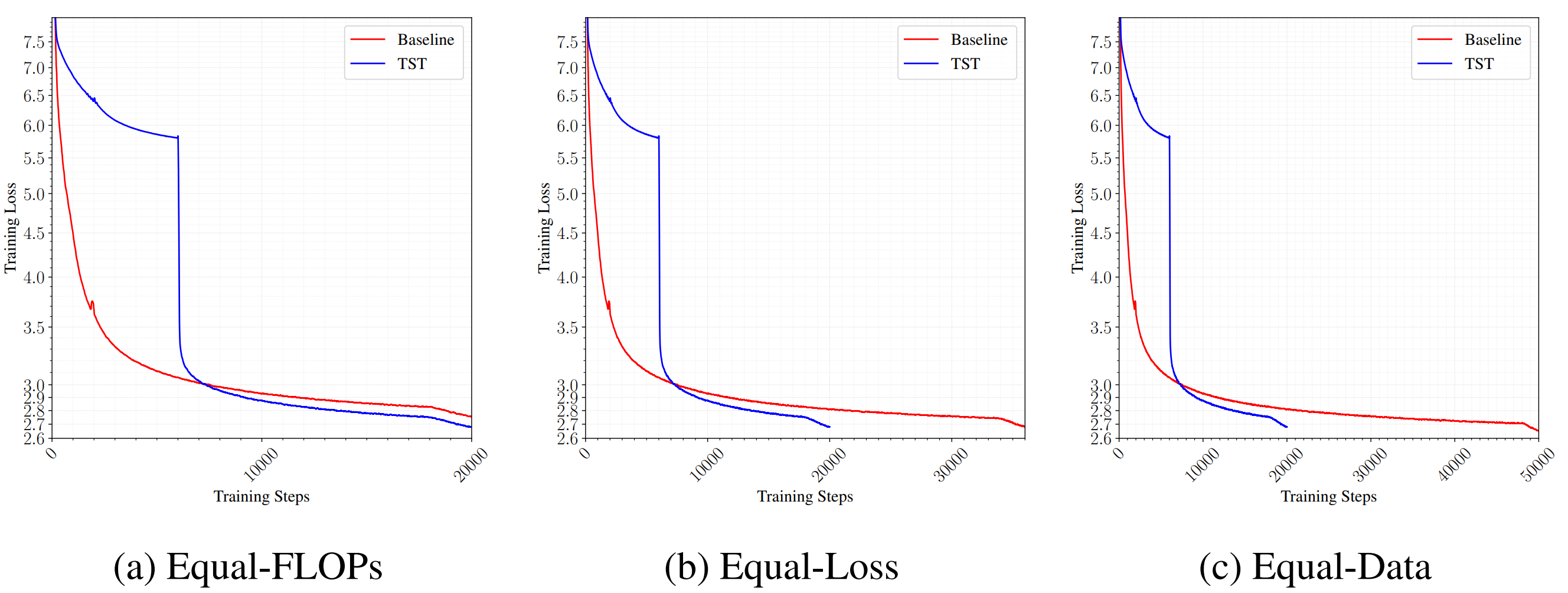
Table 1 collects the main results. B200-hours are the wall-clock proxy on our hardware. The TST-tokens column reports the number of tokens consumed during phase 1; the total-tokens column reports the full run.

Model	Params	Total steps	Bag size	Tokens (TST / total)	B200-hrs	Loss	HellaSwag	ARC-E	ARC-C	MMLU
Baseline	270M	20k	–	– / 42B	34	3.212	36.3	46.7	24.9	–
TST	270M	20k	6	75B / 105B	34	3.142	38.6	47.6	26.4	–
Baseline	270M	100k	–	– / 209B	170	3.092	40.2	47.5	26.2	–
TST	270M	100k	6	377B / 524B	170	3.048	42.6	50.3	25.5	–
Baseline	600M	20k	–	– / 42B	61	3.019	43.5	51.7	25.5	–
TST	600M	20k	6	75B / 105B	61	2.943	48.2	52.5	26.9	–
Baseline	3B	20k	–	– / 42B	247	2.808	57.6	60.6	31.9	31.2
Baseline	3B	36k	–	– / 75B	443	2.677	62.3	65.9	34.9	32.7
Baseline	3B	50k	–	– / 105B	622	2.640	63.9	67.3	36.8	33.3
TST	3B	20k	6	75B / 105B	247	2.676	62.4	66.3	36.0	32.8
Baseline	10B-A1B	125k	–	– / 1.05T	12311	2.252	70.1	73.8	46.3	37.4
TST	10B-A1B	50k	16	1.68T / 2T	4768	2.236	71.2	74.2	47.3	39.0

The pattern is consistent across scales. At 3B, TST at 20k steps matches a 36k-step baseline in final loss while using a similar wall-clock budget and producing essentially identical downstream scores. Pushing the baseline to 50k steps allows it to surpass the 20k-step TST run, which is expected: TST front-loads a fixed speedup, it does not compound indefinitely on a given budget. At 10B-A1B the speedup is cleanest because the budget is largest; the TST run reaches the baseline's final loss in under 40% of the wall-clock and improves by one point or more on each of the four evals reported. The 10B run was a single configuration rather than a cherry-picked sweep. Every downstream benchmark lands above baseline, which is a meaningfully stronger result than a loss improvement alone, given the well-known tendency of training-loss reductions to fail to transfer.

Sensitivity is documented in Figures 4 through 7 of the paper. The sweep over bag size at fixed ratio $r$ produces a U-shaped curve: below a certain $s$, the superposition regime is too similar to standard training for the throughput gain to matter; above it, the bag target becomes too lossy, and phase 2 cannot fully recover in the remaining budget. Between these extremes is a wide flat basin, which is the regime in which the method is useful. The basin's location drifts upward with model size. At 270M/42B it sits between $s = 3$ and $s = 8$; at 600M/42B between $s = 6$ and $s = 10$; at 10B/2T the configuration we ran was $s = 16$. We cannot draw a scaling law from a handful of points, but the direction is at least consistent with the hypothesis that larger models can tolerate coarser superposition. This is the dimension along which we would most like to see further study.

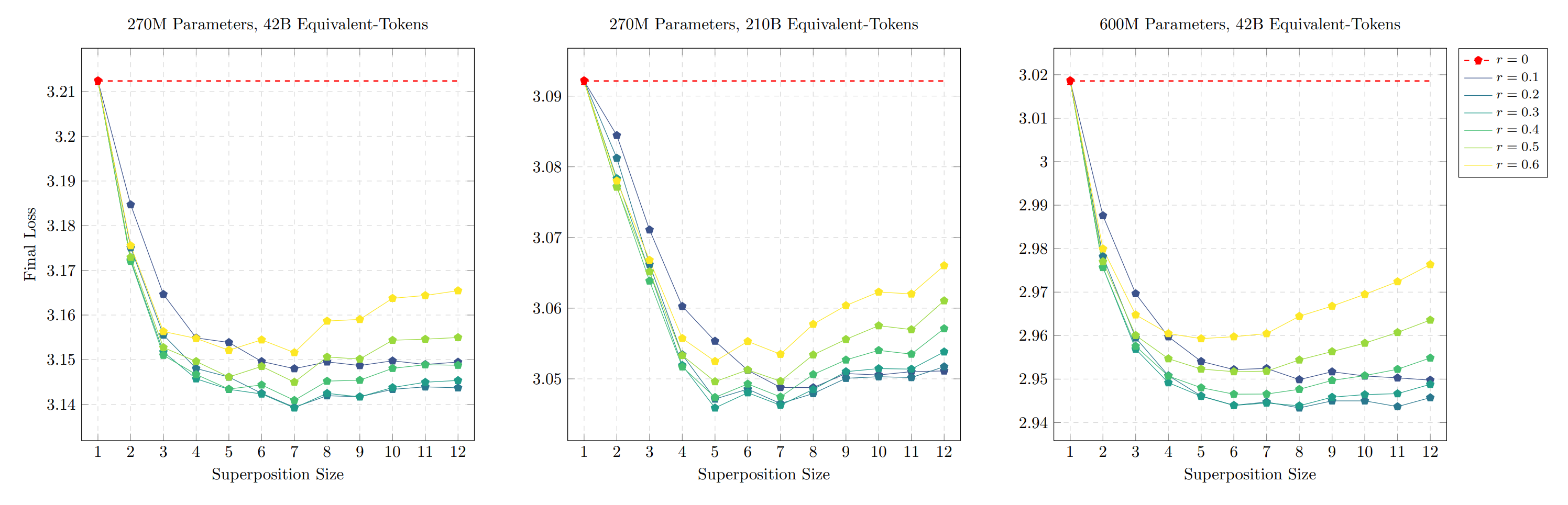
The step ratio $r$ is less sensitive. Values between 0.2 and 0.4 are close to optimal in all configurations we tested. At $r = 0$ the method reduces to the baseline; at $r \geq 0.5$ phase 2 has too few steps remaining to undo the damage that the superposition objective inflicts on the output head, and final loss degrades. Downstream evaluations track the loss curves rather than diverging from them, which is consistent with a view in which TST is not distorting the model's representations in a way that would specifically hurt transfer.

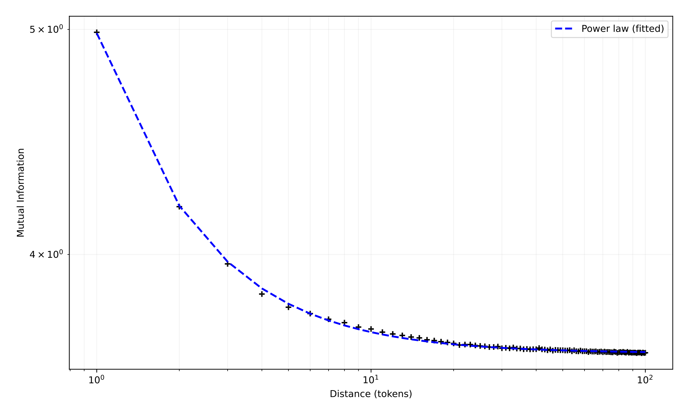
A small additional refinement concerns the weighting within the bag. In the simplest version of the loss, each of the $s$ positions in a target bag contributes equally. At larger bag sizes this is suboptimal. We find that a power-law weighting in which the $i$-th target position contributes $1/i$ to the loss produces lower final loss than uniform weighting for $s \geq 8$, while being indistinguishable at smaller $s$. The weighting is motivated by an observation due to Ebeling and Pöschel, who showed in 1994 that mutual information between pairs of English letters decays as a power law with distance. We measured the equivalent quantity for tokenized DCLM and found the same functional form, with fitted exponent $k \approx -1.25$. Weighting near targets more heavily than far ones is therefore the inductive bias consistent with the statistics of natural text, and it is the weighting that wins empirically; the coincidence struck us as worth recording.

Two mechanisms

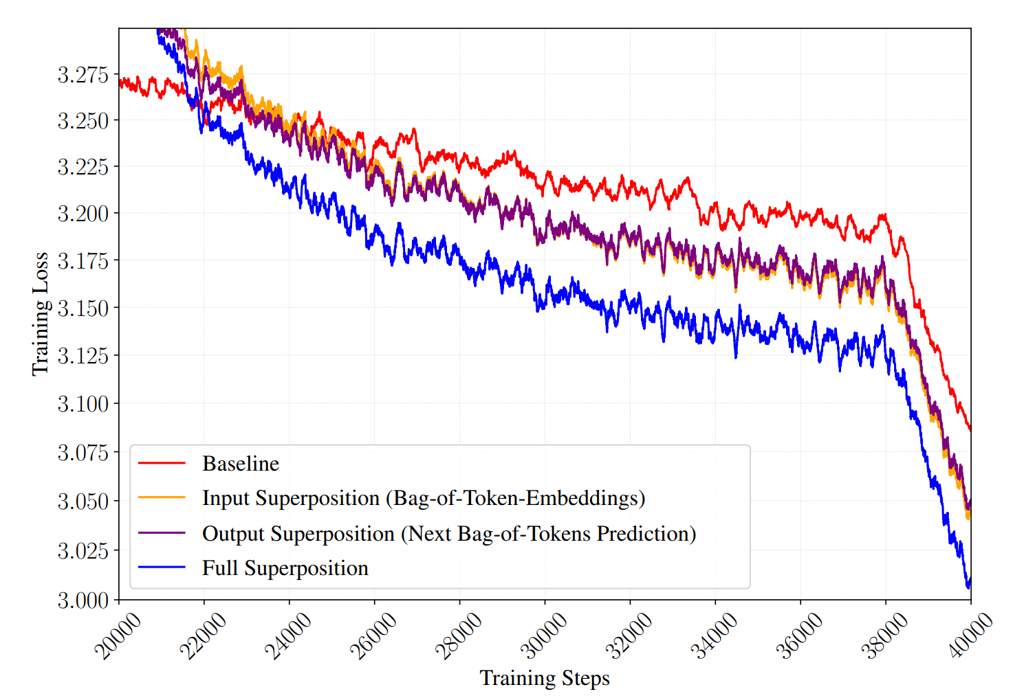
TST has two moving parts — the input-side superposition and the output-side multi-hot objective — and each can be ablated independently. Doing so shows that both, on their own, outperform the baseline, and that their effects combine approximately additively when used together (Figure 6). We read this as evidence that TST is not a single trick with two knobs but two distinct mechanisms that happen to be compatible.

The output-side mechanism is the easier of the two to place in the existing literature. Next-bag-of-tokens prediction is structurally a form of multi-token prediction, in the sense introduced by Gloeckle et al., but with weight sharing across positions: rather than $s$ independent heads predicting the $s$ future tokens, a single head predicts the mean distribution. This makes it the cheapest member of a family of methods that now includes DeepSeek-V3's cascaded MTP, Zuhri et al.'s token-order prediction, Liu et al.'s next-concept prediction, Mahajan et al.'s future-summary prediction, and a concurrent modded-nanogpt speedrun entry that proposed a similar next-bag objective with exponential weighting and a smooth phase transition rather than a hard switch. The common thread across all of these is that an auxiliary signal drawn from the near future produces a more informative gradient than the per-position one-hot target of standard next-token prediction.

What is perhaps conceptually interesting about the bag objective in particular is that it discards order information entirely within the bag. The model is not being asked which token will appear at which exact position in the next $s$ steps; it is being asked only which tokens appear at all. That this target produces a useful training signal suggests that a substantial portion of what next-token prediction is forcing the model to learn concerns the distribution of near-future tokens rather than their precise ordering, and that the two can be partially separated. Framed this way, the bag target is a form of topic modeling over a short future window, closer in spirit to the bag-of-words summarization of Luhn and the inverse document frequency of Sparck Jones than to next-token prediction. The closest recent work, as noted, is Mahajan et al.'s future-summary prediction, which also targets a compressed view of the future but attaches an auxiliary head with its own loss on top of the main NTP objective; TST instead keeps a single head and replaces the target.

The input-side mechanism is harder to place. There is no direct analogue in the recent pretraining literature, and we do not have an ablation clean enough to decisively choose between the plausible explanations. Averaging $s$ contiguous embeddings produces, in expectation, the centroid of the bag's embedding distribution, and the model is then asked to perform language modeling on a sequence of such centroids rather than on discrete tokens. One possibility is that this amounts to a form of noise reduction: the mean operator is a low-pass filter over the embedding sequence, and may damp the high-frequency variance that makes the early phase of training noisy, particularly at large $s$. A second, not mutually exclusive, possibility is that the operation implicitly regularizes the geometry of the embedding matrix. For the model to extract useful information from an averaged bag, sums of many random $s$-grams of tokens must remain separable in embedding space, which constrains the vocabulary to be laid out with sufficient angular dispersion. Under this reading the superposition phase is a regularizer on the embedding table, applied during phase 1 and inherited at phase 2.

A third framing, which we find the most suggestive though we cannot yet prove it, connects input-side TST to a growing body of work on pre-pretraining. Hu et al. show that training a language model on formal languages before natural language imparts useful inductive biases and reduces the token budget required to reach a given loss by roughly a third; Lee et al. obtain a similar effect using synthetic data generated by neural cellular automata, accelerating convergence by 1.6× with 164M pre-pretraining tokens. The recurring observation is that a first training stage conducted on a simpler distribution, one that shares coarse statistical structure with natural language without reproducing all of its complexity, can leave the model better prepared to learn from natural language in a subsequent stage. The superposition phase is such a simpler distribution, in the obvious sense that it is a coarser version of the same text. If the analogy holds, input-side TST may be interpretable as an extremely cheap instance of pre-pretraining, with the pre-pretraining corpus constructed on the fly from the real corpus by averaging. This predicts that certain attention-head circuits acquired in phase 1 should remain functional in phase 2, as they do in Hu et al.'s formal-language experiments. We have not performed that analysis, but it seems to us the most direct way to test this hypothesis.

It is worth locating this work in the broader organization of pretraining efficiency research. One can group the field into three loosely defined categories. Information-maximization methods increase the informational content of each training sample, either through improved input representations (better tokenization, $n$-gram hashing) or through richer supervision signals (auxiliary losses, multi-token prediction, order-augmented objectives). Compute-sparsity methods keep the representation fixed and reduce the FLOPs expended per token, typically by activating a subset of parameters or attending to a subset of positions. Compressive-modeling methods learn to internally compress the input representation so that fewer latent positions flow through the expensive layers. Output-side TST is a variant of the first category. Input-side TST is a variant of the third, with the distinguishing property that the compression is applied only during a first training phase and discarded afterward, so that the inference-time model retains the original tokenization and granularity. This last property is what decouples the training-time efficiency from the inference-time architecture, and is the feature of TST that we find philosophically most useful.

Limitations

The method trades compute for data. The 600M run at what we labeled a "42B equivalent-token" budget in fact consumes 105B tokens from the data loader. Under the assumption that pretraining compute is the binding constraint, as it has been for most labs through the era that produced the models underlying this paper, this trade is favorable. Under the opposite assumption, where the binding constraint is the available text rather than the available compute, TST is actively counterproductive, because it spends the corpus faster than standard training does. Kim et al. argue that the compute-bound assumption will weaken in the coming years as the open-web text available for training saturates relative to the compute budgets labs can afford to spend on it. Whether and when that transition will occur is beyond the scope of this work to predict. What we can say is that the output-only variant of TST, which preserves the auxiliary future signal but does not consume extra tokens, is the natural candidate for the data-bound regime. We have not yet benchmarked it head-to-head against multi-token prediction or order-augmented prediction, and that comparison is the most pressing follow-up we are aware of.

Two further limitations deserve mention. The experimental program includes a wide sweep at 270M and 600M, validation at 3B, and a single large-scale run at 10B-A1B. The scaling of the optimal bag size with model size is therefore supported by three data points, which is enough to indicate a trend but not enough to fit a law. Predicting the optimal TST configuration for frontier-scale pretraining would require a proper scaling study, which the existing sweep is explicitly a prelude to rather than a substitute for. Separately, during phase 1 the effective context length in the underlying text is $s$ times the sequence length processed by the transformer, so at $s = 8$ and an 8k model context the model is exposed to 64k-token spans of source text. The consequences of this exposure for long-context behavior at evaluation time are unknown, because we did not evaluate them. The most likely outcome is a small positive effect stemming from the reduced need to truncate long documents during phase 1, but this is a hypothesis rather than a result.

Negative results

For the sake of completeness, a selection of variants that we tried and that did not improve on the default recipe. We mention them because someone trying to reproduce or extend this work is likely to consider them as well.

Introducing positional encodings on the tokens prior to averaging, with the aim of preserving some amount of within-bag order information through the mean, consistently failed to help and often hurt. The invariance of the bag under permutations of its contents appears to be a structural feature of the input-side mechanism rather than a limitation of it.

Several alternative output losses were considered, including binary cross-entropy against a multi-hot target, an analogue of the token-order-prediction head of Zuhri et al., and a hinge-style ranking loss. In all cases, the simpler mean-CE formulation was more stable across settings and produced the best final loss. We suspect this is because the MCE target is more closely aligned with the standard NTP target that phase 2 will switch to, so the recovery phase has less to unlearn.

Rescaling RoPE at the phase transition, on the principle that phase 1 processes $L/s$ positions per sample while phase 2 returns to $L$, accelerated the first few thousand steps of recovery but sometimes resulted in a higher final loss. Leaving RoPE unchanged and allowing phase 2 to treat the longer effective range as new territory proved more stable across our runs.

Finally, a middle ground between single-head next-bag prediction and full $k$-head multi-token prediction, in which $s$ heads predict the $s$ positions of each bag, produced no consistent gain over the single-head MCE objective at the cost of an additional $s \cdot |V|$ parameters and an increase in implementation complexity. The simpler version is preferable.

Open questions and future work

Beyond the scaling study and the data-bound comparison already mentioned, we see two directions of interest. The first is the possibility of using the phase-1 model for something other than a warmup. By the time phase 1 ends, the model has learned an $s$-to-1 compression of the input and can decode distributions over $s$-token futures from the compressed representation. These are the characteristic operations of a speculative-decoding draft model, or of a prefix encoder in a retrieval system. Extracting an auxiliary artifact from phase 1 for use at inference time, while continuing the main training run into phase 2, would impose no additional training cost and might yield a genuinely useful inference-time component. The second is the possibility of retaining the TST head during phase 2 as an auxiliary MTP-style loss rather than discarding it at the phase boundary. The head is already trained and presumably carries information about the near-future distribution that standard NTP training does not reinforce. This is the variant that would most directly address the data-bound regime, and is also the one most compatible with the auxiliary-loss literature.

If you're interested in working on problems like this, reach out on Twitter or Discord.