NousCoder-14B: A Competitive Olympiad Programming Model

Introduction

We introduce NousCoder-14B, a competitive olympiad programming model post-trained on Qwen3-14B via reinforcement learning. On LiveCodeBench v6 (08/01/2024 - 05/01/2025), we achieve a Pass@1 accuracy of 67.87%, up 7.08% from the baseline Pass@1 accuracy of 60.79% for Qwen3-14B. We trained on 24k verifiable coding problems using 48 B200s over the course of four days.

Dataset

Following the success of Agentica x Together AI's DeepCoder-14B^[1], we use the same dataset as them. In particular, our training dataset consists of 24K problems from TACO Verified, PrimeIntellect's SYNTHETIC-1, and LiveCodeBench problems before 07/31/2024. The test dataset we use is LiveCodeBench v6 (08/01/2024–05/01/2025) consisting of 454 problems^[2]. We verified that there is no contamination between the train and test datasets.

The datasets consist entirely of "competitive programming" problems, which are code generation problems whose solutions must satisfy time and memory constraints and also pass a series of input and output test cases.

RL Environment

We use the Atropos framework to construct our RL environment.

Using the standard LiveCodeBench prompt, we prompt the model to generate Python solutions for each problem. Since each coding problem has a verifiably correct answer, we assign an outcome-based reward to each rollout of the model. In particular, we assign the following rewards:

• Reward 1 - The LLM-generated code passes all test cases supplied in the dataset for that problem. Each problem contains hundreds of test cases on average.
• Reward -1 - The LLM-generated code outputs the wrong answer, exceeds the maximum time limit of 15 seconds, or exceeds the 4GB memory limit for any of the test cases.

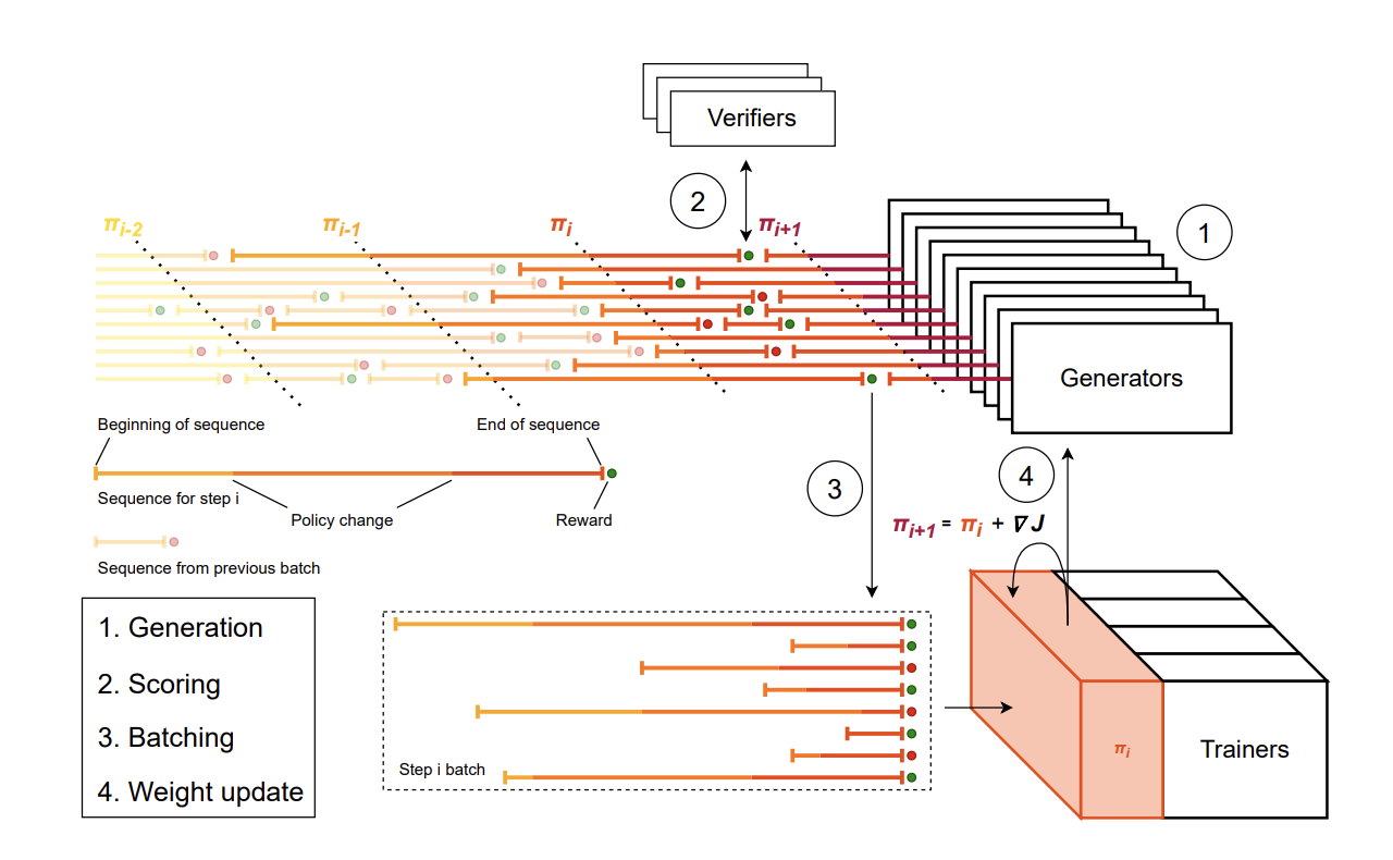
To perform sandboxed execution of code in parallel, we use Modal, an autoscaler, to help with the code verification process and to assign rewards to rollouts. We score each generation by launching a Modal container per rollout and evaluating the code on every test case for a single problem. Since problems in LiveCodeBench can have hundreds of test cases, we use Modal to prevent the resource-intensive task of evaluating LLM-generated code from competing with resources used for training and inference.

We also overlap inference and verification as shown in Figure 3. As soon as an inference worker finishes a generation, the completion is sent to a verifier (in Modal) and the inference worker immediately begins generating another completion simultaneously. For instance, assuming we have 256 maximum inference workers and 100 maximum Modal containers, one can see how pipelining inference and verification is useful so that the inference workers are not bottlenecked by Modal. By overlapping inference with verification, the evaluation process remains inference-compute-bound rather than verification-bound. Figure 3 illustrates the pipelined inference and verification process.

Parallelizing the verification process is also an interesting problem. There are three approaches for parallelization we experimented with, from coarse to fine-grained:

• One Modal container per LiveCodeBench problem. Each container evaluates multiple rollouts per problem. The number of rollouts is equivalent to the group size in Group Relative Policy Optimization (GRPO). This is the coarsest level of parallelization.
• One container per rollout. Each container evaluates multiple test cases for one rollout. This is the parallelization level we ultimately used.
• One container per test case. Rather than launching one container per problem, we experimented with a more fine-grained parallelization approach in which each container evaluated one test case for one rollout. This verification process can be further optimized by selecting the top 3-5 hardest test cases (which we heuristically determine based on the length of the test case) and evaluating them first, and if any of these test cases fail, we are done with the verification process for that rollout and no longer need to launch Modal containers for hundreds of other test cases. However, since individual container launches come with overhead in terms of time, and more importantly cost, we ultimately used a per problem, rather than per test case, parallelization approach for verification.

All of our RL environment code is open-sourced. Our grader is adapted from rllm and LiveCodeBench's implementations.

Training Setup

GRPO Algorithm and Variants

We experimented with the following three objectives: Dynamic sAmpling Policy Optimization (DAPO)^[4], Group Sequence Policy Optimization (GSPO)^[5], and a modified version of GSPO we call GSPO+. If the rewards are given by $\{R_i\}_{i=1}^G$, the advantages for all objectives are given by

$$\hat A_i = \frac{R_i - \text{mean}(R)}{\text{std}(R)}$$

The DAPO objective is given by

$$J_{DAPO}(\theta) = \mathbb{E}\left[\frac{1}{\sum_{i=1}^G |o_i|} \sum_{i=1}^G \sum_{j=1}^{|o_i|} \min\left(r_{i,t}(\theta)\hat A_i, \text{clip}(r_{i,t}(\theta), 1-\epsilon_{low}, 1+\epsilon_{high}) \hat A_i\right)\right]$$

where the $r_{i,t}(\theta) = \frac{\pi_\theta(o_{i,t}|q,o_{i,<t})}{\pi_{old}(o_{i,t}|q,o_{i,<t})}$ represents the token-level importance ratio and $o_i$ is the generation for the $i$-th rollout.

As a brief summary, the DAPO objective introduces several key improvements over the vanilla GRPO objective:

• Clip-higher. This encourages more exploration for low probability tokens.
• Token-level policy gradient loss. Regardless of the length of the generation, each token is rewarded or penalized equally with respect to the policy gradient.
• Dynamic sampling. Discard groups that consist entirely of incorrect or correct solutions because the advantage is zero and therefore offers no information for training.

The GSPO objective is given by

$$J_{GSPO}(\theta) = \mathbb{E}\left[\frac{1}{G} \sum_{i=1}^G \min\left(s_i(\theta)\hat A_i, \text{clip}(s_i(\theta), 1-\epsilon_{low}, 1+\epsilon_{high}) \hat A_i\right)\right]$$

where the sequence-level importance ratio is given by

$$s_i(\theta) = \frac{\pi_\theta(o_i|q)}{\pi_{old}(o_i|q)} = \exp\left(\frac{1}{|o_i|} \sum_{j=1}^{|o_i|} \log \frac{\pi_\theta(o_{i,j}|q,o_{i,<j})}{\pi_{old}(o_{i,j}|q,o_{i,<j})}\right)$$

From the GSPO paper:

The unit of optimization objective should match the unit of reward. Since the reward is granted to the entire sequence, applying off-policy correction at the token level appears problematic. This motivates us to forego the token-level objective and explore utilizing importance weights and performing optimization directly at the sequence level^[5].

The GSPO+ objective is given by

$$J_{GSPO+}(\theta) = \mathbb{E}\left[\frac{1}{\sum_{i=1}^G |o_i|} \sum_{i=1}^G |o_i| \min\left(s_i(\theta)\hat A_i, \text{clip}(s_i(\theta), 1-\epsilon_{low}, 1+\epsilon_{high}) \hat A_i\right)\right]$$

The only difference between the GSPO to the GSPO+ objective is that policy gradients per token are now equally weighted regardless of the length of the generation, just like the DAPO objective.

Context Length	Qwen3-14B (No RL)	DAPO	GSPO	GSPO+
40,960	60.79%	63.35%	63.13%	63.06%
81,920	60.79%	67.87%	66.26%	66.52%

Table 1: Pass@1 model performance with different RL algorithms and context lengths.

Context Length	Qwen3-14B (No RL)	DAPO	GSPO	GSPO+
40,960	75.11%	79.52%	78.19%	77.53%
81,920	75.11%	78.41%	78.63%	79.07%

Table 2: Pass@G model performance with different RL algorithms and context lengths.

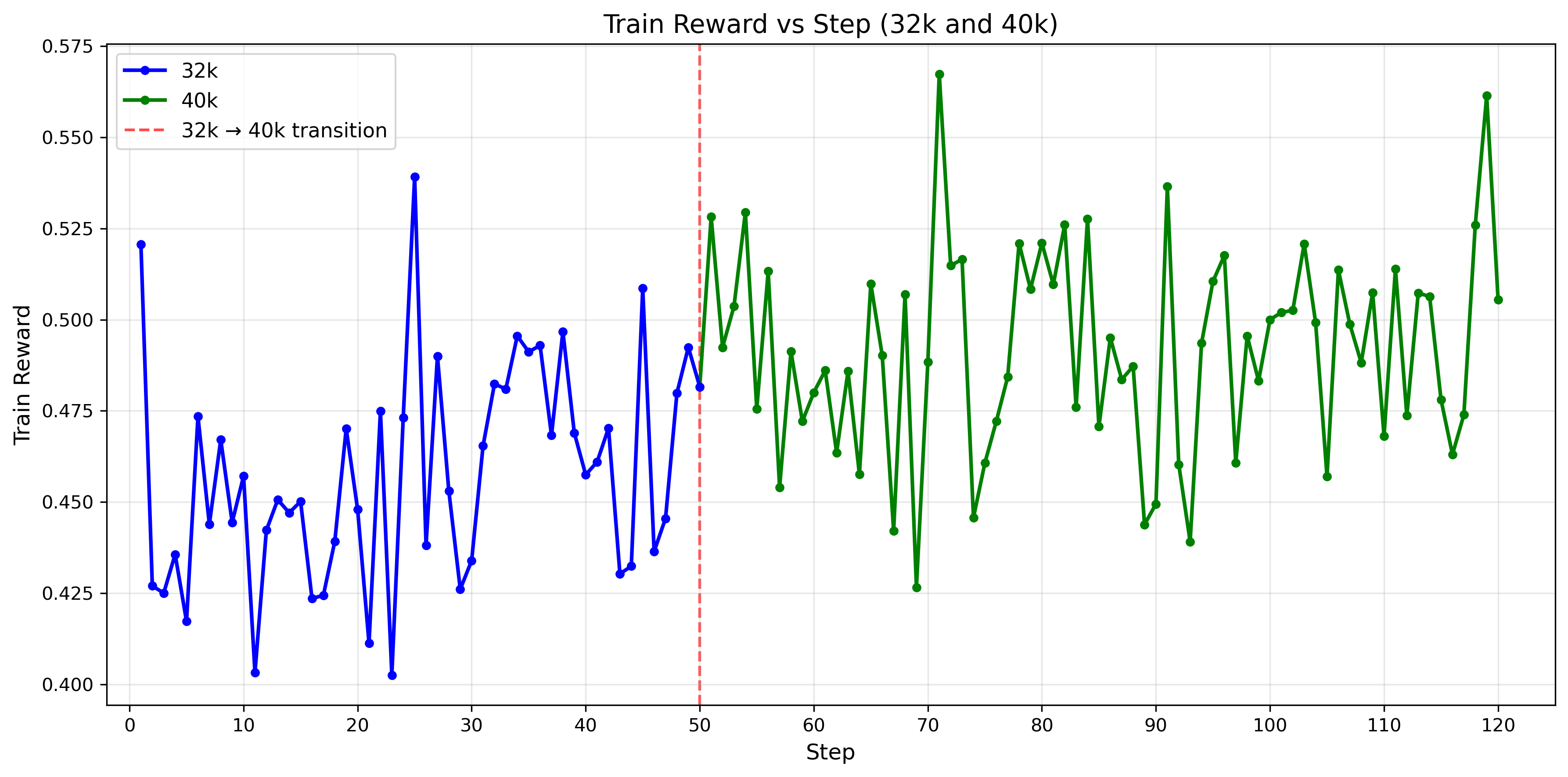
Looking at Table 1, we find that the DAPO objective performs the best by only a small margin. We also found that throughout our training process, all objectives performed similarly, so we only show the training curves for the DAPO objective as shown in Figure 4. More comprehensive training curves can be found in our WandB dashboard. Surprisingly, the specific objective used does not appear to have a significant impact on the model's performance.

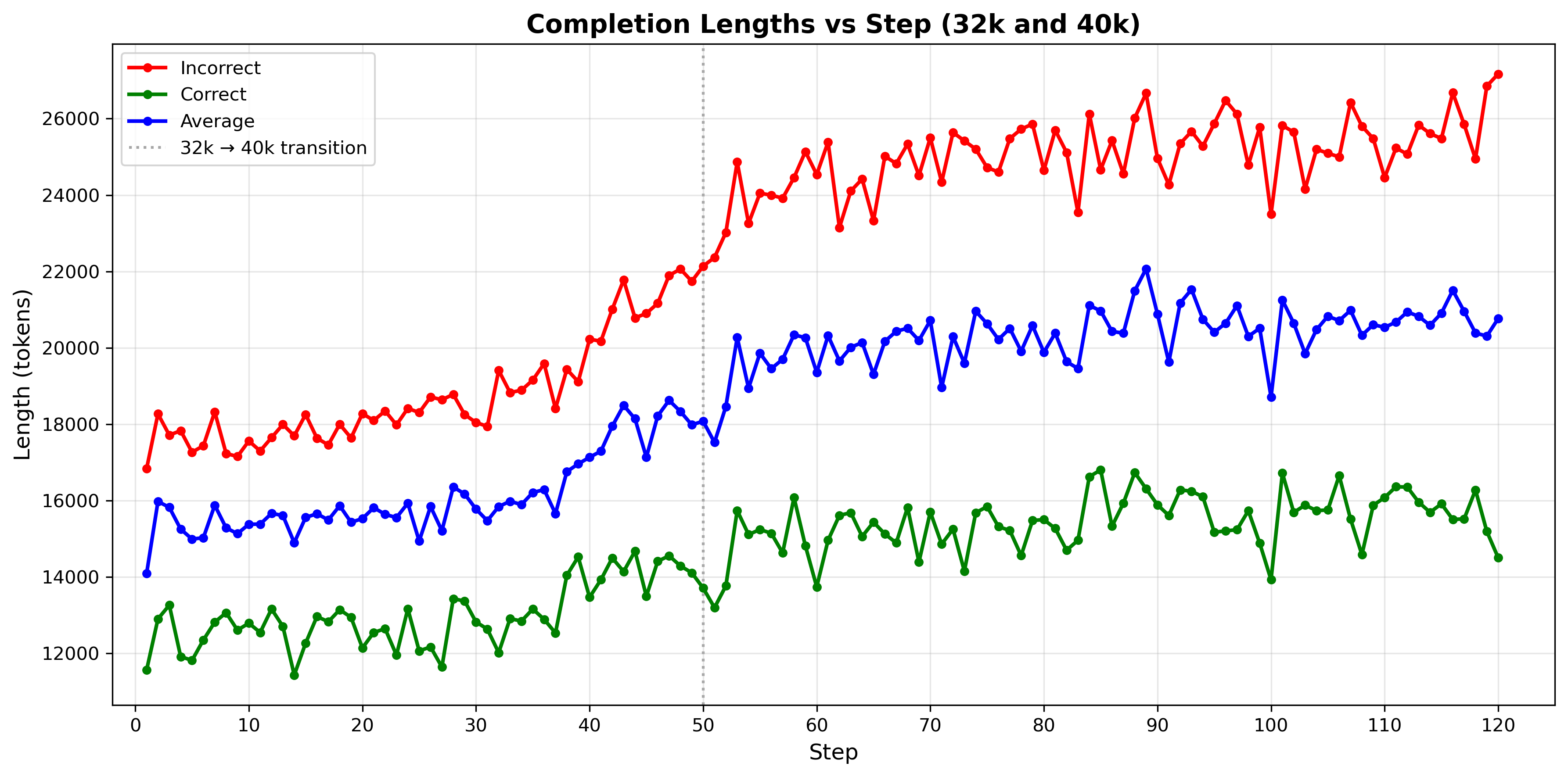
The primary motivation for experimenting with DAPO and GSPO+ was to try to address the issue of length bias where shorter correct solutions and longer incorrect solutions are preferred. When we initially observed the GSPO training curves (which turns out to be nearly identical to the DAPO and GSPO+ training curves), we saw that incorrect solution lengths were consistently longer and increased more over training steps compared to correct solution lengths as shown in Figure 5. As a result, the maximum context window would be quickly saturated. However, our algorithmic changes ultimately did not solve this length bias issue.

Hyperparameters

Hyperparameter	Value
Learning Rate	$10^{-6}$
KL Divergence Coefficient	$0$
Group Size	$8$
Batch Size (Sequences Per Batch)	$1024$
$k$ value: PPO-off-policy-k	$4$
$k$ value: PipelineRL-k	$3$
Temperature (Training / Evaluation)	$1.0 / 0.6$
Top-p (Training / Evaluation)	$1.0 / 0.95$
DAPO Clip Ratio (low/high)	$0.2 / 0.28$
GSPO Clip Ratio (low/high)	$3 \times 10^{-4} / 4 \times 10^{-4}$

Table 3: Hyperparameters used in the training process.

Note that the batch size, PPO-off-policy-k, and PipelineRL-k hyperparameters are all related to the asynchronous RL training setup, which we will discuss later on.

Iterative Context Extension

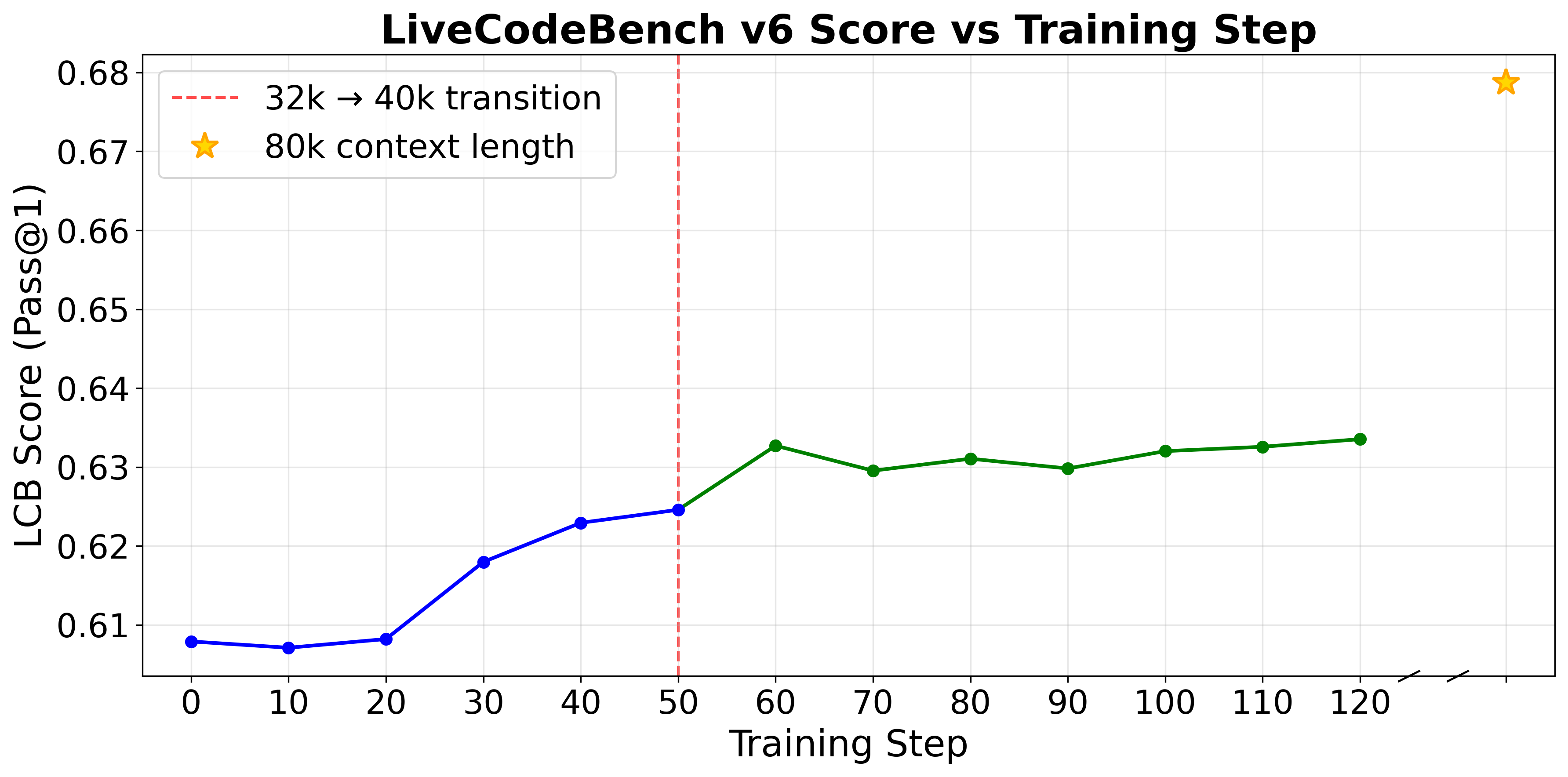
As in the DeepCoder blog^[1], we also adopt an iterative context lengthening approach in which we first train the model using a context window of 32k, and then train the model using the maximum Qwen3-14B context window of 40k as shown in Figure 6. This incentivizes the model to first learn at a shorter context window and then extend it to the maximum context window.

We also use the overlong filtering approach from DAPO^[4]. Whenever the model generation exceeds the maximum context window, we override the previously computed advantage for that rollout and set its advantage to zero. Therefore, the model does not receive a penalty for generating a solution that exceeds the maximum context window. As a result, we're able to see significant improvement when scaling up the context window during test-time.

We select the highest performing model, in terms of LiveCodeBench score evaluated at 40k context, trained at 32k context and use it as the starting point for training at 40k context. Then, we select the highest performing model at 40k context and use YaRN context extension to evaluate the model with a 80k context window.

Additional Training Tricks

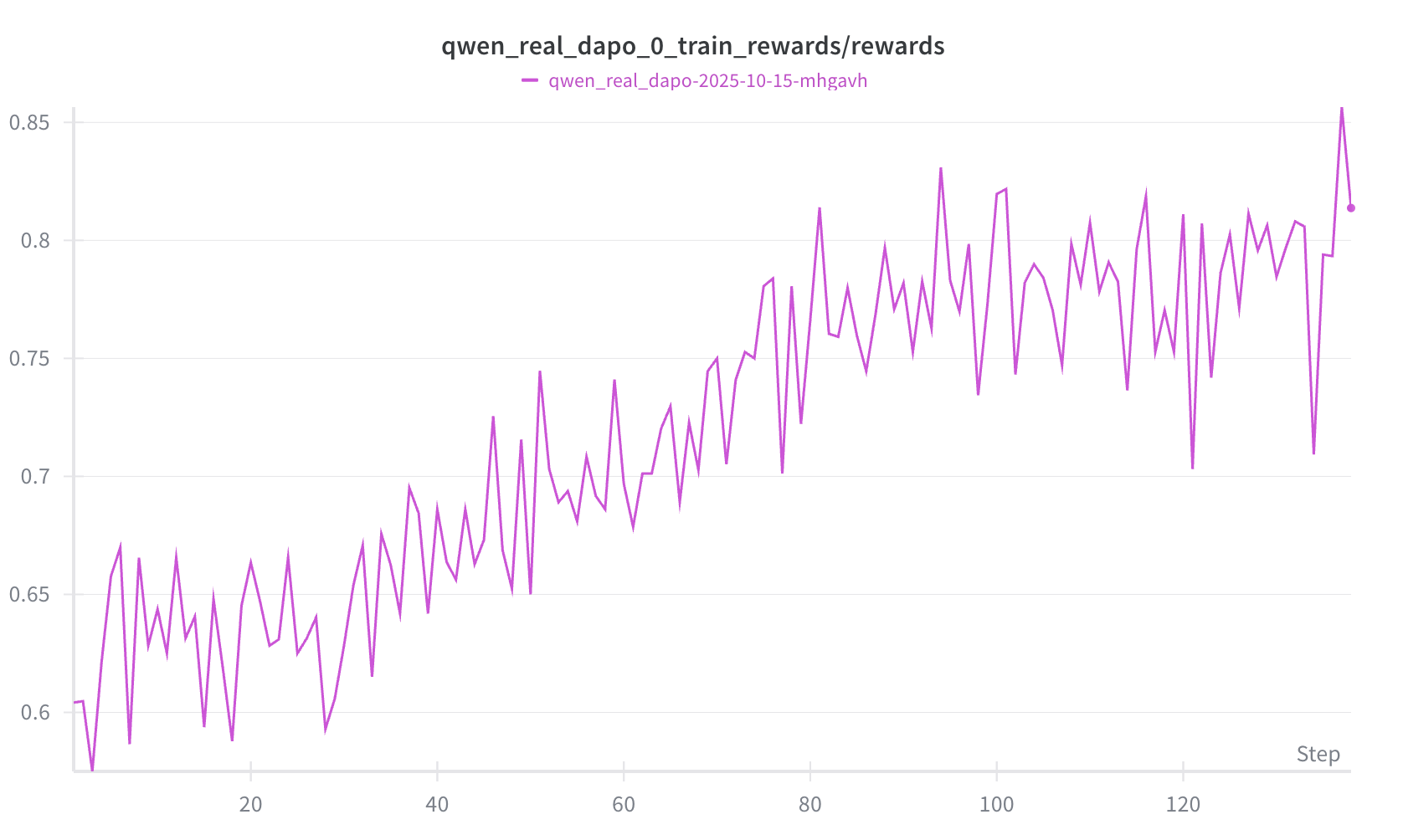
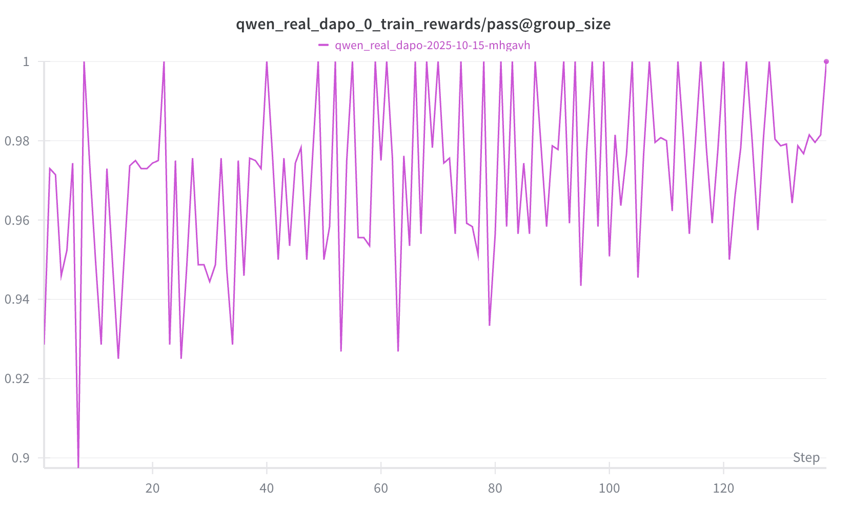
We present an experimental technique that was extremely useful for fast iteration and served as an initial test for correctness in choosing hyperparameters, algorithms, and so forth. We selected a fixed subset of 64 problems that the base Qwen3-14B model would achieve a $0 < \text{pass@G} < 1$ where $G$ is the group size. In other words, out of $G$ rollouts, the model solves the problem at least once but less than $G$ times, and we would train the model using only these problems. The expectation is that the train rewards should noticeably increase. If we use the entire training dataset, the improvement in training reward is less noticeable and takes longer to observe as shown in Figure 4. Figure 6 shows a successful example of this technique, where setting our KL divergence coefficient to zero allowed us to observe noticeable improvement in training reward, whereas our previous experiments yielded no noticeable improvement in training reward when we used a positive KL divergence term. Figure 7 shows that all training examples have at least one correct solution generated by the model.

Additionally, we found that around 10k out of the 24k problems in the training dataset would be consistently solved by the Qwen3-14B model (all rollouts would pass). Therefore, we can filter out these problems offline, prior to training, since they provide no gradient information during training. Then, since the model improves over many epochs of training, we can do online filtering to remove training examples once the model achieves 100% pass@1 on a particular problem. This method significantly reduces inference time.

Asynchronous RL Training

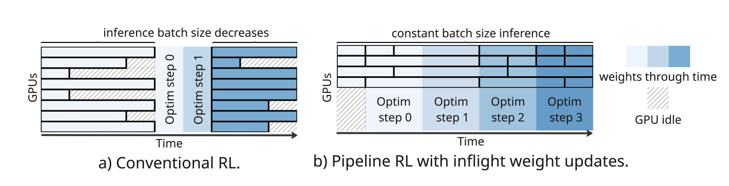
To maximize hardware efficiency, we employ a distributed asynchronous RL setup as shown in Figure 8. Our setup closely resembles that of PipelineRL^[6]. In particular:

The Pipeline RL method differs from Conventional RL in two aspects: (1) running training and generation in parallel asynchronously, and (2) updating the generation weights after every optimizer step in-flight, i.e. without stopping the sequence generation^[6].

We define the batch size $B$ as the number of rollouts the inference workers collect before sending them to the trainer, which conducts an optimizer step using these $B$ sequences and updates the inference model weights. Since inference workers are continuously streaming rollouts along with the trainer, we want to prevent the inference workers from collecting rollouts too far ahead of the trainer. From the notation in ScaleRL^[7], we employ PipelineRL-$k$, where $k$ indicates the maximum difference between the expected optimizer step for in-progress rollouts and the current optimizer step of the trainer. In other words, at any point in time, the number of active rollouts plus the number of completed rollouts not yet processed by the trainer should never exceed $k \times B$. This helps control how far off-policy the rollouts are.

Furthermore, within a batch we can also take optimizer steps, which ScaleRL calls PPO-off-policy-$k$. In other words, we take $k$ optimizer steps per batch: each gradient step processes $\frac{B}{k}$ rollouts.

Given the asynchronous nature of the training setup, we need to carefully handle importance sampling ratios and modify the objective. To motivate this, we will first discuss the objective within a synchronous RL context. As shown by Yao et al.^[8] and Liu et al.^[9], even when the parameters between the trainer $\pi_{learner}$ and inference model $\pi_{sampler}$ are the same, the usage of highly optimized inference engines like vLLM and SGLang can lead to significant differences in the token probabilities. To fix this issue, they propose an objective with truncated importance sampling:

$$\mathbb{E} \left[ \sum_{i=1}^G \text{TIS}(a_i)\min\left(\frac{\pi_{learner}(a_i|q)}{\pi_{learner,old}(a_i|q)}\hat A_t, \text{clip}\left(\frac{\pi_{learner}(a_i|q)}{\pi_{learner,old}(a_i|q)}, 1-\epsilon_{low}, 1+\epsilon_{high}\right)\hat A_t\right)\right]$$

where $\pi_{learner,old}$ is the training policy before the off-policy gradient steps are taken for a batch and $\text{TIS}(a_i)$ is the truncated importance sampling ratio given by

$$\text{TIS}(a_i) = \min\left(C, \frac{\pi_{learner,old}(a_i|q)}{\pi_{sampler}(a_i|q)}\right).$$

In our asynchronous RL setup, we adopt this exact objective. Note that a single rollout may be sampled by multiple $\pi_{sampler}$ policies since the model will update in-flight without interrupting generation. If $\pi_{learner,old}$ represents the policy at the start of $k$ gradient steps in PPO-off-policy-$k$, then it is clear that $\pi_{sampler}$ and $\pi_{learner,old}$ differ not because of the trainer-inference implementation mismatch when model weights are theoretically the same, but the two policies are now legitimately different. While the objective shown above is for sequence-level importance sampling, it can be easily adapted to token-level importance sampling for DAPO.

Future Work

Given more time, we would like to try three main things:

• Train models with larger context windows and find a better way to control response lengths. We found that our response lengths would quickly saturate the context window.
• Multi-turn RL. When our RL environment grades a rollout, it is possible to give the model more feedback than just a final binary reward. Most competitive programming problems have public test cases visible to the programmer, and executing model code on these public test cases can yield valuable information such as compilation errors, time and memory violations, and incorrect answers. All this feedback can be used to guide the model's response in a multi-turn RL setting before the final binary reward is given.
• Problem generation and self-play for competitive programming. Is it possible to train a model to not only solve problems but also to generate solvable problems? How does an LLM know if the problem is solvable? Humans are great at generating interesting and useful problems for other competitive programmers, but it appears that there still exists a significant gap in LLM capabilities in creative problem generation. Once synthetic problem generation is solved, however, self-play becomes a very interesting direction.

Closing Remarks

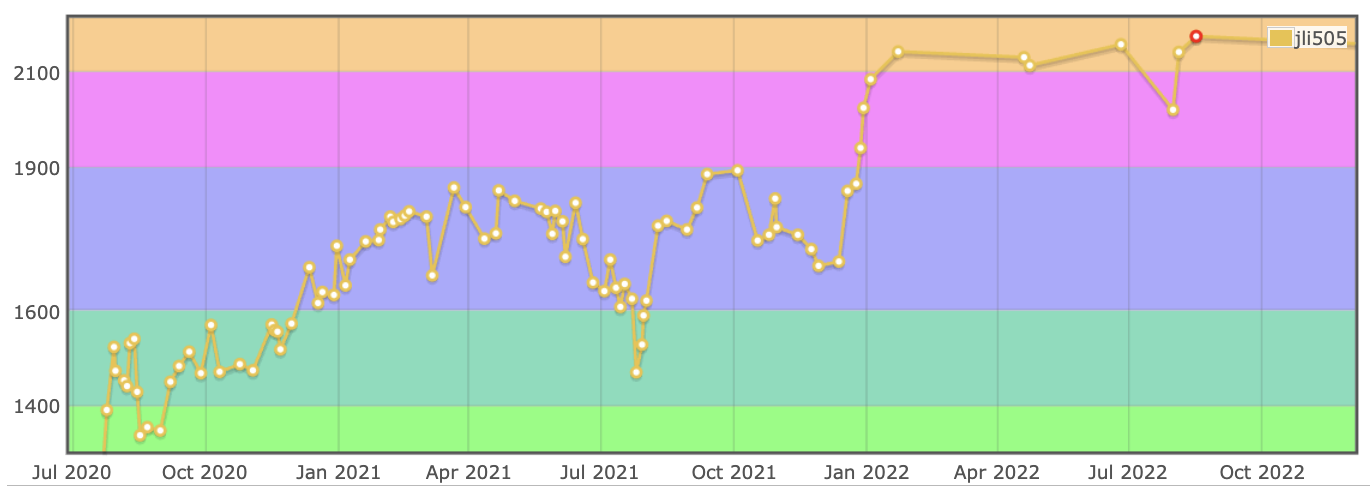
One of the most remarkable aspects of this work was being able to compare the model's capabilities to my own capabilities as a former competitive programmer. Based on some very rough estimations to determine the model's Codeforces rating from its LiveCodeBench score, the model's comparable Codeforces rating improved from the 1600-1750 range to the 2100-2200 range. Figure 9 shows my own Codeforces rating history. Between the ages of 14 and 16, it took me nearly two years of sustained effort to make that same rating jump, something the model accomplished in just four days of training. Watching that final training run unfold was quite a surreal experience.

However, I solved around 1k problems to achieve that rating jump, whereas the model needed 24k; I was clearly more sample efficient than the model, which brings us to an interesting discussion on data efficiency. These 24k problems encompass a significant portion of all readily available, verifiable competitive programming problems in a standardized dataset format, and the total number of competitive programming problems on the Internet is roughly the same order of magnitude. This suggests that within the competitive programming domain, we have approached the limits of high-quality data. Moreover, one of the hallmarks of a competitive programmer is the ability to also create interesting and useful problems for other competitive programmers, but LLMs still struggle in this domain. More broadly, this serves as a reflection on modern scaling paradigms; while it is possible to continue scaling compute, data is becoming increasingly finite; it appears that some of the most important research that needs to be done in the future will be in the areas of synthetic data generation and data efficient algorithms and architectures.

Acknowledgements

I would like to thank my mentor, Roger Jin, Dakota Mahan, Teknium, and others at the Nous Research team for their invaluable support throughout this project. I would also like to thank Together AI and Agentica for their immensely helpful blog posts on DeepCoder-14B. Finally, thank you to Modal and Lambda for their generous support by providing me with credits.

References

1. Michael Luo et al.
   DeepCoder: A Fully Open-Source 14B Coder at O3-mini Level.
   Notion Blog, 2025. ↩
2. Naman Jain et al.
   LiveCodeBench: Holistic and Contamination Free Evaluation of Large Language Models for Code.
   arXiv:2403.07974, 2024. ↩
3. Mistral AI.
   Magistral.
   arXiv:2506.10910, 2025. ↩
4. Qiying Yu et al.
   DAPO: An Open-Source LLM Reinforcement Learning System at Scale.
   arXiv:2503.14476, 2025. ↩
5. Chujie Zheng et al.
   Group Sequence Policy Optimization.
   arXiv:2507.18071, 2025. ↩
6. Alexandre Piché et al.
   PipelineRL: Faster On-policy Reinforcement Learning for Long Sequence Generation.
   arXiv:2509.19128, 2025. ↩
7. Devvrit Khatri et al.
   The Art of Scaling Reinforcement Learning Compute for LLMs.
   arXiv:2510.13786, 2025. ↩
8. Feng Yao et al.
   Your Efficient RL Framework Secretly Brings You Off-Policy RL Training.
   Notion Blog, 2025. ↩
9. Jiacai Liu et al.
   When Speed Kills Stability: Demystifying RL Collapse from the Training-Inference Mismatch.
   Notion Blog, 2025. ↩
10. LiveCodeBench Team.
    LiveCodeBench Leaderboard.
    2025. ↩