Lighthouse Attention

TL;DR. A selection-based hierarchical attention that runs the same forward+backward pass ~17× faster than standard attention at 512K context on a single B200, and delivers a 1.4–1.7× end-to-end pretraining speedup at 98K context. Q, K, V are pooled symmetrically across an L-level pyramid; per-head $\ell_2$ norms pick a small dense sub-sequence; FlashAttention runs on the gather — no custom sparse attention kernel, no straight-through estimator, no auxiliary loss. After the sparse stage, a brief standard attention resume converts the checkpoint back into a dense attention model: every recovered run matches or beats dense-from-scratch at the same token budget. Validated at 530M Llama-3, 16k optimiser steps, 50B tokens, with 1M-token training across 32 B200s under context parallelism.

Long-context pretraining is bottlenecked by attention's quadratic compute cost. FlashAttention shaves the constants, but the wall is still there: you train at the contexts you can afford.

We introduce Lighthouse Attention, a selection-based hierarchical attention that pools queries, keys and values symmetrically across a multi-resolution pyramid, scores every pyramid entry with a parameter-free function, and keeps the selection logic outside the attention kernel. The expensive step in the forward pass is FlashAttention on a small dense sub-sequence. The same kernel runs at training and inference, and we inherit every upstream FlashAttention improvement unchanged.

The code is at github.com/ighoshsubho/lighthouse-attention.

Two design decisions

Most prior work in this space (NSA, HISA, InfLLM-v2, DSA, MoBA) makes two design decisions that quietly matter for training.

Asymmetry. Queries stay at full resolution; only keys and values are pooled. The hierarchy serves as a compressed addressable memory rather than a multi-scale representation.

Architectural entanglement. Selection lives inside the attention kernel. The carefully optimised dense attention kernels that modern tensor cores accelerate can't be reused; every sparse method ships its own kernel.

There is also a concern specific to training. An inference-time sparse method is at most as good as its dense backbone: the sparse substitution is evaluated only against the dense forward. A training-time sparse method has to survive a harder test: once training is done, will the model still be a competent dense-attention model? If not, it has just trained a specialist of its own approximation.

We treat that question as the central correctness check.

The method

Symmetric pooling. Q, K and V all get pooled by the same factor at every level of the hierarchy. A pooled query at level $\ell$ lives in the same representation space as a pooled key at level $\ell$. This is the choice that turns the dense-attention call from $O(N \cdot S \cdot d)$ to $O(S^2 \cdot d)$ at training time.

Parameter-free scoring. Each pyramid entry gets two scalar scores: the $\ell_2$ norm of its query projection, and the $\ell_2$ norm of its key projection. There is no learned scorer head, no auxiliary loss, no Gumbel-softmax, no straight-through estimator. The projections are encouraged to be useful when selected, not to score well at selecting. A dilated softmax-attention scorer is a strictly stronger signal — it sees QK interactions, the norm scorer doesn't — so our results are a lower bound on what selection-based training can give.

Selection outside the kernel. Once top-K is decided, we gather the chosen entries into a contiguous, causally-sorted dense sub-sequence and run FlashAttention on it. The expensive step at training time is the same dense-attention kernel the dense baseline uses; forward and backward are bit-for-bit identical to a dense Transformer's.

The four stages

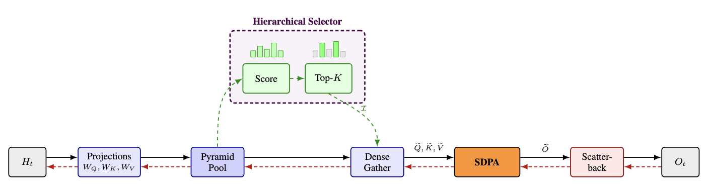
A Lighthouse attention layer replaces standard scaled dot-product attention with four stages that surround, but do not modify, the attention kernel.

Three small interactive panels make each stage concrete.

(i) Pyramid pool

Average-pool Q, K, V symmetrically into an L-level pyramid with pooling factor $p$:

$$ Q^{(\ell)} = \mathrm{Pool}_{\mu}(Q), \quad K^{(\ell)} = \mathrm{Pool}_{\mu}(K), \quad V^{(\ell)} = \mathrm{Pool}_{\mu}(V), \quad \ell = 0, 1, \ldots, L-1 $$

Level 0 is the full sequence; level $\ell$ has $N/p^{\ell}$ tokens, each summarising $p^{\ell}$ base positions. The viz uses $N = 16$, $L = 3$, $p = 2$ (16 base tokens fanning up to 8 + 4 pooled summaries), so you can see exactly which base positions a coarse cell is responsible for.

(ii) Top-K cascade

Compute per-head $\ell_2$ norms across all levels for queries and keys, and select jointly:

$$ s^{(QK)}_{\ell,i} = \|Q^{(\ell)}_i\|_2, \qquad s^{(KQ)}_{\ell,i} = \|K^{(\ell)}_i\|_2 $$

$$ \mathcal{I} = \mathrm{TopK}\!\left( \{ s^{(QK)}_{\ell,i},\, s^{(KQ)}_{\ell,i} : (\ell, i) \in \mathcal{P} \},\, k \right) $$

The viz walks the cascade coarse-to-fine: top-K at the coarsest level, descend into the children of the survivors, top-K again, descend, and at the base level keep everything. Selected cells brighten with a gold ring; rejected cells dim and pick up a red ring.

A coarse entry at level $\ell$ summarises $p^{\ell}$ contiguous base positions. If we threw away every rejected coarse entry, the survivors at level $\ell$ would no longer tile the base sequence: there would be gaps over the positions whose coarse summary didn't make the cut, and whose finer descendants weren't selected either (since selection is inherited from selected parents). Those gaps are exactly what would force a sparse-aware causal mask later on.

We avoid that by keeping rejected coarse entries in the buffer alongside the selected ones. Each level $\ell$ contributes at most $p \cdot K$ entries (K from top-K, plus a small p-factor of causal-boundary book-keeping). After we sort the gathered triples by base-sequence position, the resulting sub-sequence is topologically causal with no holes: the standard $S \times S$ lower-triangular causal mask just works, and the attention kernel never sees a sparse layout.

(iii) Attention as a black box, then scatter-back

Gather the surviving (Q, K, V) triples into a contiguous sub-sequence of length

$$ S = N / p^{L-1} + (L - 1) \cdot p \cdot K $$

run ordinary FlashAttention on it,

$$ \tilde{O} = \mathrm{Attn}(\tilde{Q}, \tilde{K}, \tilde{V};\, \tilde{M}) $$

and then scatter each output entry back to the $p^{\ell}$ base positions it represents, with a shift of $p^{\ell} - 1$ (so a coarse summary of positions $[a, a + p^{\ell} - 1]$ writes to $[a + p^{\ell} - 1, a + 2p^{\ell} - 2]$: the causal boundary again). Accumulation runs in one of two kernels: a default non-deterministic fp-atomic, and a deterministic integer-atomic that is 1.2–2× slower. The deterministic kernel is intended only for reproducing results; the fp-atomic is the default.

Most of the implementation is two new files plus ~600 lines of edits on top of upstream torchtitan: every step that might have wanted a custom sparse kernel is instead a torch.gather followed by a torch.sort and then ordinary FlashAttention.

Training recipe

The trained model has to remain a competent dense-attention model after sparse training, so the recipe is two-stage:

• Stage 1 (Lighthouse). Train for the majority of the budget with Lighthouse selection enabled.
• Stage 2 (SDPA-resume). Resume the stage-1 checkpoint with selection disabled; continue training under standard attention for a brief tail. Same optimiser state, same dataloader continuation.

If the sparse training signal hollowed out the model's dense-attention ability, stage 2 would fail to recover. If it didn't, stage 2 will smoothly converge to a model competitive with a dense-from-scratch run.

Across three split points (10k+6k, 11k+5k, 12k+4k of total 16k steps), every recovered Lighthouse run matches or beats the dense-from-scratch baseline at the same 16,000-step / ~50B-token budget. At each resume point the loss spikes by 1.12–1.57 nats as the model is first asked to use dense attention it was not trained against, then recovers within roughly 1k–1.5k SDPA steps.

This is the load-bearing claim of the paper: sparse training does not compromise the model's ability to use full attention at inference, at no additional token cost over dense-from-scratch.

Ablations

The ablation grid (530M Llama-3, 16k optimiser steps, 8×B200 single node unless the row says CP):

Configuration	Scorer	LH steps	Total steps	Tokens	B200-Hrs ↓	Tok/s (k) ↑	Final Loss ↓
SDPA baseline (ctx = 98K)	n/a	n/a	16k	50.3B	303.2	45.6	0.7237
SDPA recoverability (L=3, p=2, k=6144, ctx = 98K)
LH → SDPA (12k+4k)	Dilated	12k	16k	50.3B	214.7	74.7	0.7102
LH → SDPA (11k+5k)	Dilated	11k	16k	50.3B	219.6	75.4	0.7001
LH → SDPA (10k+6k)	Dilated	10k	16k	50.3B	228.0	75.0	0.6980
Hyperparameter ablations (ctx = 98K)
L=3, p=2, k=1536	Dilated	10k	16k	50.3B	203.9	93.9	0.6825
L=3, p=4, k=1536	Dilated	10k	16k	50.3B	197.2	99.5	0.6881
L=3, p=8, k=1536	Dilated	10k	16k	50.3B	206.2	92.1	0.6828
L=4, p=2, k=1536	Dilated	10k	16k	50.3B	200.2	96.4	0.6978
L=5, p=2, k=1536	Dilated	10k	16k	50.3B	201.5	96.3	0.6991
L=3, p=2, k=2048	Dilated	10k	16k	50.3B	208.1	90.9	0.6880
L=3, p=2, k=4096	Dilated	10k	16k	50.3B	215.7	83.5	0.6951
CP training (L=3, p=4)
k=1536, ctx = 98K, CP=2, DP=4	Norm	10k	16k	100.7B	208.3	91.8	0.6903
k=2048, ctx = 98K, CP=2, DP=4	Norm	10k	16k	100.7B	210.9	89.2	0.6928
k=4096, ctx = 256K, CP=8, DP=1	Norm	10k	16k	1.07T	1300.3	48.9	0.6721

Every recovered Lighthouse run beats the dense-from-scratch baseline (final loss 0.6980–0.7102 vs 0.7237) at the same token budget, while saving 75–106 B200-hours: a 1.40× to 1.69× wall-clock speedup.

Stage-1 throughput sustains 84–126k tokens/s/GPU across the ablation grid versus ~46k for dense SDPA. Lighthouse pays for itself entirely in stage 1; the SDPA-resume tail runs the same kernel as the baseline and matches its throughput.

The pyramid hyperparameters are forgiving. $L \in \{3, 4, 5\}$ and $p \in \{2, 4, 8\}$ all land within ~0.02 nats of each other; the choice is mostly a throughput / memory-reach trade-off, not a quality knife-edge.

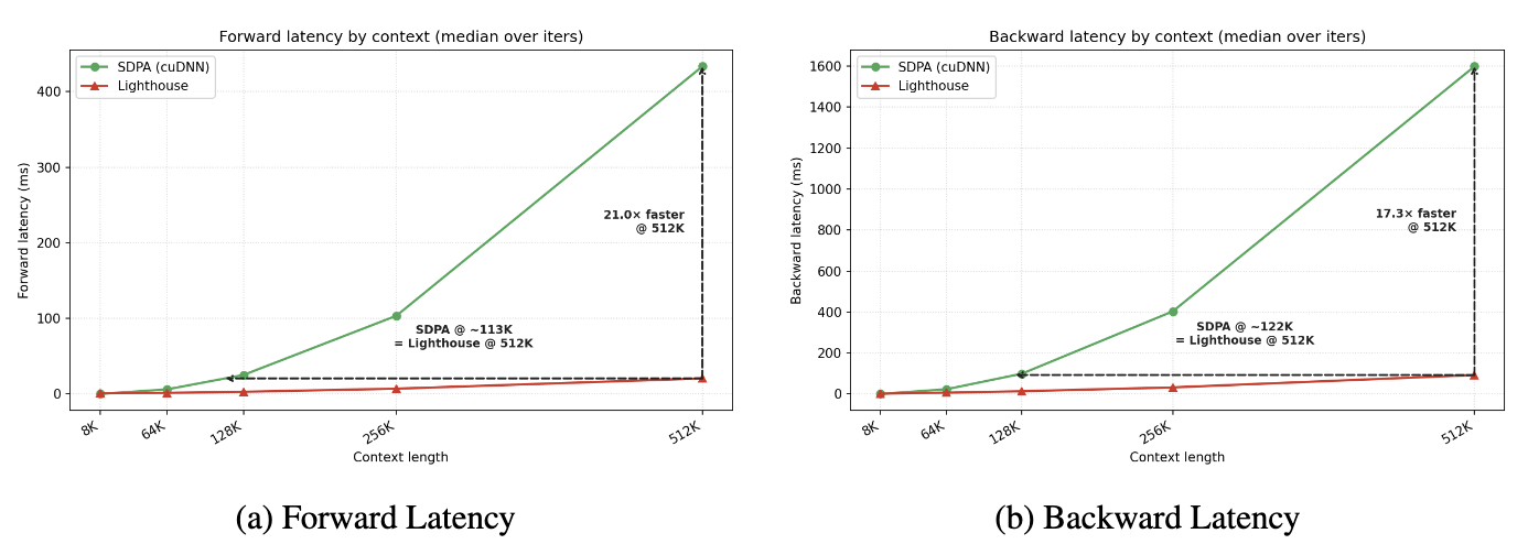
Scaling

At short contexts the two curves track each other (the constant overhead of pyramid pool + selection dominates); past the crossover point the SDPA curve climbs quadratically while Lighthouse stays close to linear in $N$ at fixed $K$. The 1.4×–1.7× end-to-end training speedup at 98K context in the ablation table is what falls out of this gap once you fold in everything else a step does (FSDP, optimizer, dataloader, scatter-back).

Long context

Beyond about 100K context our 530M architecture OOMs on a single B200 regardless of attention method, so for the long-context regime we run Lighthouse under context parallelism (CP). Pyramid pooling, scoring, and top-K all run shard-locally; the gathered sub-sequence is dense, so it participates in ring attention with no sparse-aware collectives.

This is what makes the CP path tractable. Lighthouse's selection output is a contiguous tensor; methods whose attention call expects sparse indices can't express ring rotation without engineering specific to the sparse layout. With Lighthouse, the ring rotates a dense sub-sequence and just works.

CP introduces a small ring-rotation overhead (about 10% in per-rank throughput vs the single-device extrapolation) and supports 1M-token training across 32 Blackwell GPUs (4 nodes, CP degree 8) with no changes to the inner attention kernel.

Setup

These are 530M Llama-3 models trained for 16,000 optimiser steps over ~50B tokens: small enough to sweep the ablation grid quickly, large enough to land the central correctness claim cleanly. For long-context retrieval we ran a simplified passkey test: a single digit hidden in synthetic alphanumeric filler, scored on a one-token argmax over the ten digit tokens. Three of four Lighthouse runs match or beat the dense-from-scratch baseline on that test.

Limitations

Symmetric Q/K/V pooling presumes all queries co-occur in one forward pass; autoregressive decoding violates this. We rely on the dense-SDPA resumption to convert Lighthouse weights into an inference-ready model.

The gathered sub-sequence cost is $\Theta(S^2 \cdot d)$: sub-quadratic in $N$ at fixed $K$, but not strictly linear. Regimes where $K$ must scale with $N$ to maintain recall remain uncharacterised.

Open questions

• Asymmetric sparse resumption. Replace dense-SDPA resume with an inference-oriented asymmetric sparse target (DSA, NSA, HISA, MoBA) so the converted checkpoint is natively serveable.
• Adaptive selection budget. Per-layer or per-head $K$ allocation instead of a single fixed $K$.
• Beyond text. Vision, audio, and video have natural multi-scale structure that fits the pyramid.
• Serving integration. Continuous batching, speculative decoding, and KV-cache management for the converted inference model.

Code

Reference implementation as a single patch on top of upstream torchtitan plus two new source files:

github.com/ighoshsubho/lighthouse-attention

Configs are organised by ablation axis (topk/, pool/, levels/, scorer/, cp/); the patch supports three scorer variants (norm, dilated, gla) selectable from your toml, and the CP path requires the norm scorer.

Paper: Long Context Pre-Training with Lighthouse Attention (arXiv:2605.06554).